Basic CML processing workflow
[1]:
import numpy as np
import matplotlib.pyplot as plt
import matplotlib as mpl
import tqdm
import xarray as xr
import pandas as pd

import pycomlink as pycml
Load example data and do preprocessing
We load the example data from one NetCDF file which contains the time series of 500 CMLs over 10 days. If you want to use your own data, e.g. from a CSV file, look at the respective example notebook for how to get started.
[2]:
data_path = pycml.io.examples.get_example_data_path()

cmls = xr.open_dataset(data_path + '/example_cml_data.nc')
cmls
[2]:
<xarray.Dataset> Size: 254MB
Dimensions:           (time: 15840, cml_id: 500, channel_id: 2)
Coordinates:
  * time              (time) datetime64[ns] 127kB 2018-05-10 ... 2018-05-20T2...
  * cml_id            (cml_id) <U3 6kB '0' '1' '2' '3' ... '497' '498' '499'
    length            (cml_id) float64 4kB ...
    site_a_latitude   (cml_id) float64 4kB ...
    site_a_longitude  (cml_id) float64 4kB ...
    site_b_latitude   (cml_id) float64 4kB ...
    site_b_longitude  (cml_id) float64 4kB ...
  * channel_id        (channel_id) <U9 72B 'channel_1' 'channel_2'
    frequency         (cml_id, channel_id) float64 8kB ...
    polarization      (cml_id, channel_id) <U1 4kB ...
Data variables:
    rsl               (channel_id, cml_id, time) float64 127MB ...
tsl (channel_id, cml_id, time) float64 127MB ...Have a quick look at the data of one CML
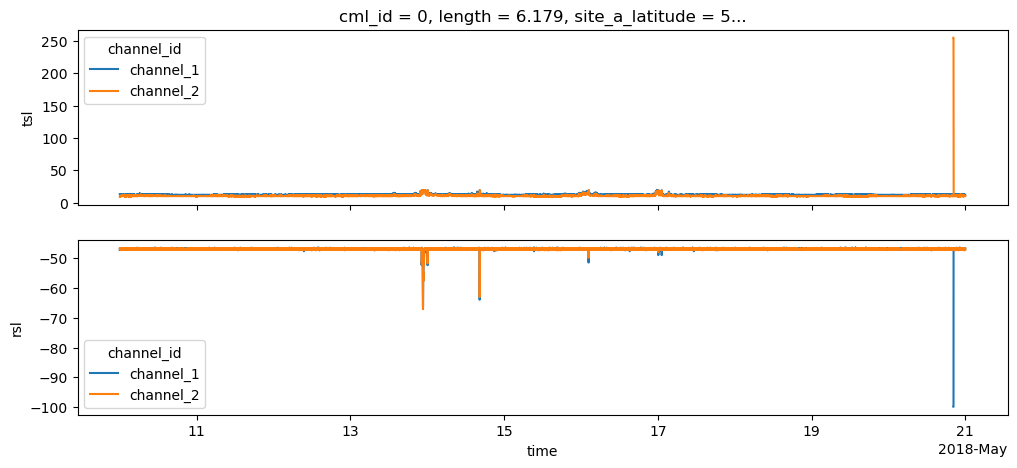
We store each CML as item of a list because we want to do the processing per CML.
In the plot, note that there are some outliers. These correspond to fill values, which we get rid of in the next step.
[3]:
cml_list = [cmls.isel(cml_id=i) for i in range(len(cmls.cml_id))]
[4]:
fig, axs = plt.subplots(2, 1, sharex=True, figsize=(12,5))
cml_list[0].tsl.plot.line(x='time', ax=axs[0])
cml_list[0].rsl.plot.line(x='time', ax=axs[1])
axs[0].set_xlabel('')
axs[1].set_title('');
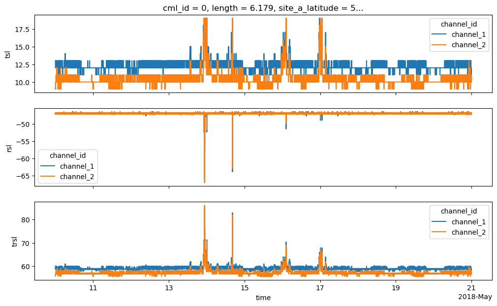
Set default and fill values to NaN and calculate TRSL
TRSL is the transmitted signal level minus the received signal level and represents the total path loss along the CML.
[5]:
for cml in cml_list:
    cml['tsl'] = cml.tsl.where(cml.tsl != 255.0)
    cml['rsl'] = cml.rsl.where(cml.rsl != -99.9)
    cml['trsl'] = cml.tsl - cml.rsl
We can now also see TSL and RSL withouth the fill values that we removed.
Also note that TRSL changes during weak attenuation events stem mostly from TSL changes because this CML has automatic transmission power control (ATPC) which tries to keep RSL constant as long as possible by increasing TSL when path-attenuation occurs.
[6]:
fig, axs = plt.subplots(3, 1, sharex=True, figsize=(12,7))
cml_list[0].tsl.plot.line(x='time', ax=axs[0])
cml_list[0].rsl.plot.line(x='time', ax=axs[1])
cml_list[0].trsl.plot.line(x='time', ax=axs[2])
axs[0].set_xlabel('')
axs[1].set_xlabel('')
axs[1].set_title('')
axs[2].set_title('');
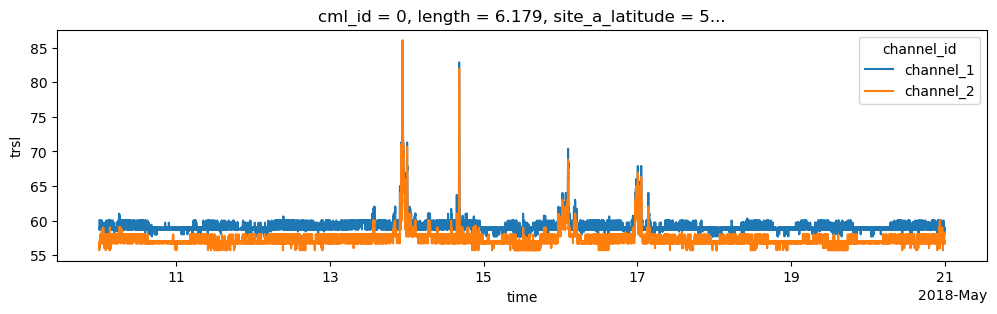
Interpolate short gaps in TRSL
Our CML data might have data gaps. These gaps can stem from outages of the data acuqisition or from blackout gaps. If they stem from a blackout gap, there are better methods than linear interpolation. See the notebook Blackout gap detection example for more details.
Here we stick to a simple linear interpolatoin of a maximum gap width of 5 minutes.
[7]:
for cml in cml_list:
    cml['trsl'] = cml.trsl.interpolate_na(dim='time', method='linear', max_gap='5min')
[8]:
cml = cml_list[0].copy() # make a copy here to not change the CML dataset in the list over which we want to iterate later
cml.trsl.plot.line(x='time', figsize=(12,3));
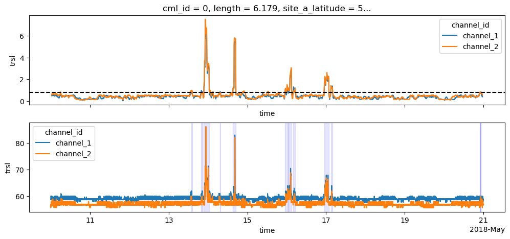
Do simple wet-dry classification using a rolling standard deviation
This is the most basic way of doing a wet-dry classification. The crucial part here is to find the optimal threshold. To keep this example short, we use a standard value of 0.8 which is more or less suitable for most CML time series. But please note, that this threshold should be adapted to the noisiness of the individual CML time series, e.g. as in Graf et al. 2020 to get the good performance for CML rainfall estimation.
[9]:
threshold = 0.8

roll_std_dev = cml.trsl.rolling(time=60, center=True).std()
cml['wet'] = cml.trsl.rolling(time=60, center=True).std() > threshold
[10]:
fig, axs = plt.subplots(2, 1, figsize=(12,5), sharex=True)

roll_std_dev.plot.line(x='time', ax=axs[0])
axs[0].axhline(threshold, color='k', linestyle='--')

cml.trsl.plot.line(x='time', ax=axs[1]);

# Get start and end of dry event
wet_start = np.roll(cml.wet, -1) & ~cml.wet
wet_end = np.roll(cml.wet, 1) & ~cml.wet

# Plot shaded area for each wet event
for wet_start_i, wet_end_i in zip(
    wet_start.isel(channel_id=0).values.nonzero()[0],
    wet_end.isel(channel_id=0).values.nonzero()[0],
):
    axs[1].axvspan(cml.time.values[wet_start_i], cml.time.values[wet_end_i], color='b', alpha=0.1)

axs[1].set_title('');
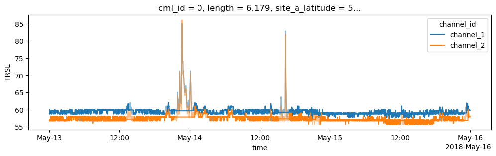
Determine baseline
[11]:
cml['baseline'] = pycml.processing.baseline.baseline_constant(trsl=cml.trsl, wet=cml.wet, n_average_last_dry=5)

fig, ax = plt.subplots(figsize=(12,3))

cml.trsl.sel(time=slice('2018-05-13', '2018-05-15')).plot.line(x='time', alpha=0.5)
plt.gca().set_prop_cycle(None)
cml.baseline.sel(time=slice('2018-05-13', '2018-05-15')).plot.line(x='time');
plt.gca().set_prop_cycle(None)
plt.ylabel('TRSL');
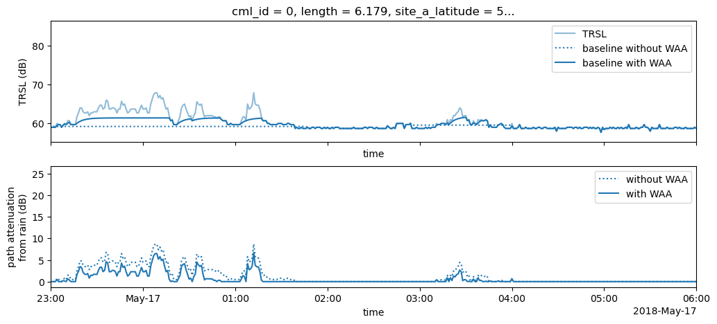
Perform wet antenna estimation and compare to uncorrected baseline
[12]:
cml['waa'] = pycml.processing.wet_antenna.waa_schleiss_2013(
    rsl=cml.trsl,
    baseline=cml.baseline,
    wet=cml.wet,
    waa_max=2.2,
    delta_t=1,
    tau=15,
)
[13]:
fig, axs = plt.subplots(2, 1, figsize=(12,5), sharex=True)

plt.sca(axs[0])
cml.isel(channel_id=0).trsl.plot.line(x='time', alpha=0.5, label='TRSL')
plt.gca().set_prop_cycle(None)
cml.isel(channel_id=0).baseline.plot.line(x='time', linestyle=':', label='baseline without WAA');
plt.gca().set_prop_cycle(None)
(cml.baseline + cml.waa).isel(channel_id=0).plot.line(x='time', label='baseline with WAA');
plt.ylabel('TRSL (dB)')
axs[0].legend()

# estimate WAA and correct baseline
cml['A'] = cml.trsl - cml.baseline - cml.waa
cml['A'].values[cml.A < 0] = 0
cml['A_no_waa_correct'] = cml.trsl - cml.baseline
cml['A_no_waa_correct'].values[cml.A_no_waa_correct < 0] = 0

plt.sca(axs[1])
cml.A_no_waa_correct.isel(channel_id=0).plot.line(x='time', linestyle=':', label='without WAA');
plt.gca().set_prop_cycle(None)
cml.A.isel(channel_id=0).plot.line(x='time', label='with WAA');
plt.ylabel('path attenuation\nfrom rain (dB)');
axs[1].set_title('');
axs[1].legend()

axs[1].set_xlim(pd.to_datetime('2018-05-16 23:00:00'), pd.to_datetime('2018-05-17 06:00:00'));
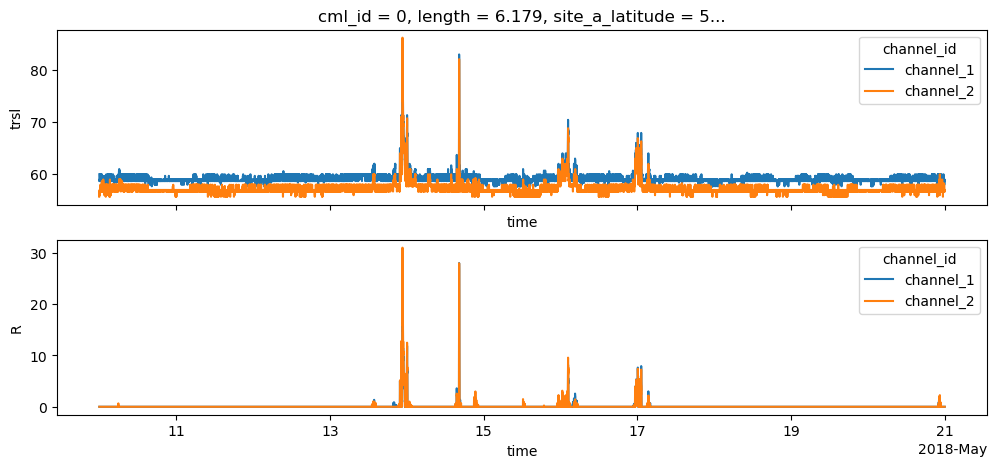
Calculate rain rate
[14]:
cml['R'] = pycml.processing.k_R_relation.calc_R_from_A(A=cml.A, L_km=float(cml.length), f_GHz=cml.frequency/1e9, pol=cml.polarization)
[15]:
fig, axs = plt.subplots(2, 1, figsize=(12,5), sharex=True)
cml.trsl.plot.line(x='time', ax=axs[0])
cml.R.plot.line(x='time', ax=axs[1])
axs[1].set_title('');
Now do the whole processing for all CMLs
[16]:
for cml in tqdm.tqdm(cml_list):
    cml['wet'] = cml.trsl.rolling(time=60, center=True).std(skipna=False) > 0.8

    cml['wet_fraction'] = (cml.wet==1).sum() / len(cml.time)

    cml['baseline'] = pycml.processing.baseline.baseline_constant(
        trsl=cml.trsl,
        wet=cml.wet,
        n_average_last_dry=5,
    )
    cml['waa'] = pycml.processing.wet_antenna.waa_schleiss_2013(
        rsl=cml.trsl,
        baseline=cml.baseline,
        wet=cml.wet,
        waa_max=2.2,
        delta_t=1,
        tau=15,
    )
    cml['A'] = cml.trsl - cml.baseline - cml.waa

    # Note that we set A < 0 to 0 here, but it is not strictly required for
    # the next step, because calc_R_from_A sets all rainfall rates below
    # a certain threshold (default is 0.1) to 0. Some people might want to
    # keep A as it is to check later if there were negative numbers.
    cml['A'].values[cml.A < 0] = 0

    cml['R'] = pycml.processing.k_R_relation.calc_R_from_A(
        A=cml.A, L_km=float(cml.length), f_GHz=cml.frequency/1e9, pol=cml.polarization
   )
100%|██████████████████████████████████████████████████████████████████████████████████████████████████████████████████████████████████████████████████████████████████████████████████████████████████████████████████████████████████| 500/500 [00:11<00:00, 42.68it/s]
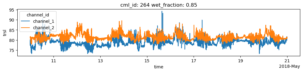
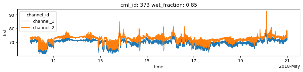
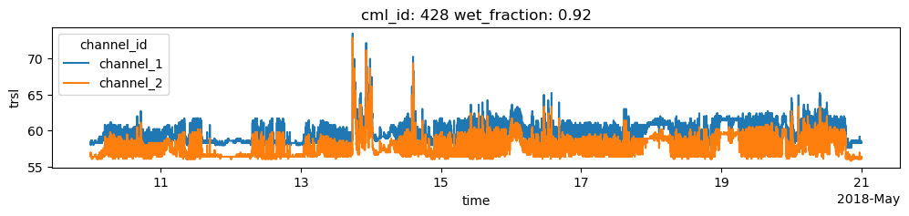
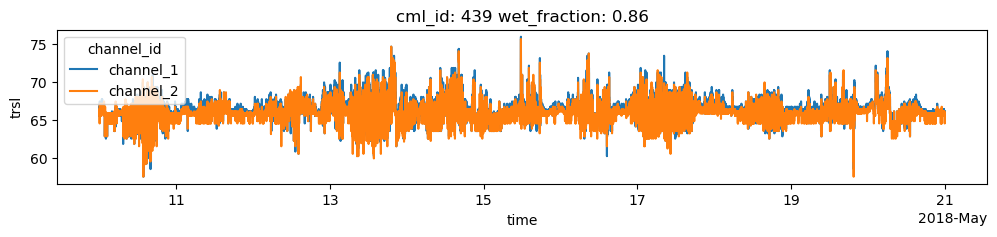
Find CMLs that show erratic behavior
Find the CMLs that have a very high ratio of wet/dry data. For the 10-day dataset that is used here and for central-European climate, a ratio higher than 0.3 can be considered very unlikely, i.e. it is unlikely that it was rainy for 30% of the one-minute data points within the 10-day period.
For the plots below, we use a higher threshold 0.8 to only plot a small number of CMLs, but find those that show very strong erratic behavior during dry periods.
[17]:
for cml in cml_list:
    if cml.wet_fraction > 0.8:
        cml.trsl.plot.line(x='time', figsize=(12,2))
        plt.title(f'cml_id: {cml.cml_id.values} wet_fraction: {cml.wet_fraction.values:0.2f}')
        plt.show()
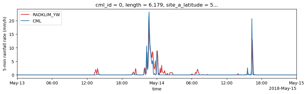
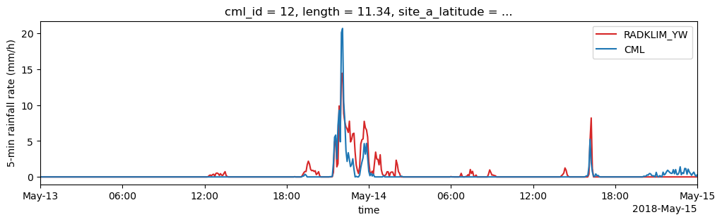
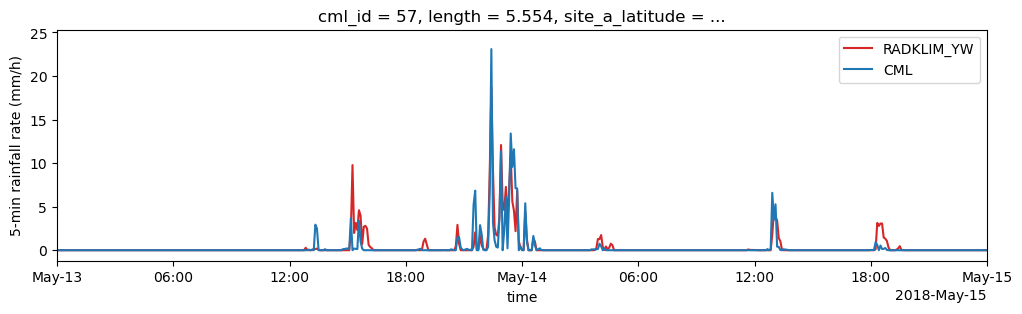
Compare derived rain rates with reference data
As reference, path-averaged rain rates along the CMLs paths from RADKLIM-YW are provided. This data has a temporal resolution of 5 minutes. First, we compare one CML timeseries aggregated to five minutes individually against its reference timeseries. Then we resample all cml data und prepare a scatterplot between CML and reference data. Finally some metrics are claculated. (for simplicity only channel 1 is evaluated here)
[18]:
path_ref = xr.open_dataset(data_path + '/example_path_averaged_reference_data.nc')
[19]:
for i in [0, 12, 57]:
    # Plot reference rainfall amount (converted to 5-minute rainfall rate)
    (path_ref.sel(cml_id=cml_list[i].cml_id).rainfall_amount * 12).plot(
        label="RADKLIM_YW", color='C3', figsize=(12,3)
    )
    # Plot 5-minute mean rainfall rates from CMLs
    (cml_list[i].sel(channel_id="channel_1").R.resample(time="5min").mean()).plot(
        x="time", label="CML", color='C0'
    )

    plt.xlim(pd.to_datetime('2018-05-13'), pd.to_datetime('2018-05-15'))
    plt.ylabel('5-min rainfall rate (mm/h)')
    plt.legend();
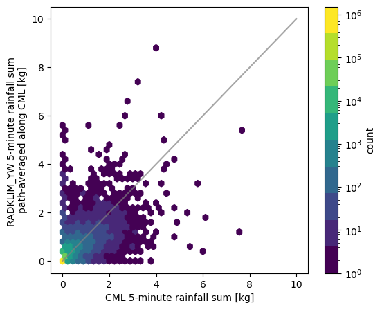
Aggregate the CML data to 5 minute rainfall sums and concat the indiviudal CML xarray.Datasets to one joint xarray.Dataset for the comparison with the reference.
[20]:
ds_cmls = xr.concat(cml_list, dim='cml_id')
[21]:
rainsum_5min = ds_cmls.sel(channel_id="channel_1").R.resample(time="5min").sum() / 60

fig, ax = plt.subplots(figsize=(6, 5))
hx = ax.hexbin(
    rainsum_5min.values.T.flatten(),
    path_ref.rainfall_amount.values.flatten(),
    mincnt=1,
    bins="log",
    gridsize=45,
    extent=(0, 10, 0, 10),
    cmap=plt.get_cmap('viridis', 10),
)
ax.plot([0, 10], [0, 10], color='gray', alpha=0.7)
ax.set_xlabel('CML 5-minute rainfall sum [kg]');
ax.set_ylabel('RADKLIM_YW 5-minute rainfall sum \npath-averaged along CML [kg]');
cbar = fig.colorbar(hx)
cbar.set_label('count')
Calculate several performance metrics. rainfall_threshold_wet defines the threshold below which a timestep is considered as dry.
[22]:
metrics = pycml.validation.stats.calc_rain_error_performance_metrics(
    rainsum_5min.values.T.flatten(),
    path_ref.rainfall_amount.values.flatten(),
    rainfall_threshold_wet=0.1)

[print(f'{metric}={value}') for metric, value in zip(metrics._fields, metrics)];
pearson_correlation=0.6834012664635292
coefficient_of_variation=8.646148144620074
root_mean_square_error=0.06931875505595712
mean_absolute_error=0.011793011431390889
R_sum_reference=12630.237843307716
R_sum_predicted=24069.548867923764
R_mean_reference=0.007973670239267292
R_mean_predicted=0.015195489416887425
false_wet_rate=0.02548173384389654
missed_wet_rate=0.1581905678537055
false_wet_precipitation_rate=0.2328701841190468
missed_wet_precipitation_rate=0.25619966292398055
rainfall_threshold_wet=0.1
N_all_pairs=1584000
N_nan_pairs=7
N_nan_reference_only=0
N_nan_predicted_only=7
Create rainfall fields via IDW interpolation
First, we combine all CMLs into one xarray.Dataset because this is the way our interpolator function requires its input. In addtion, resampling to the desired temporal aggregation is also much faster when done for one large Dataset instead of iterating over the Datasets of the individual CMLs to do the resampling.
We resample the CML rain rate data from 1 minute resolution with raw time stamps (which are, in our case, not located at the full minutes) to 1-hour averages from which we want to interpolat the maps.
[23]:
cmls_R_1h = ds_cmls.R.resample(time='1h', label='right').mean().to_dataset()
cmls_R_1h
[23]:
<xarray.Dataset> Size: 2MB
Dimensions:           (cml_id: 500, channel_id: 2, time: 264)
Coordinates:
  * cml_id            (cml_id) <U3 6kB '0' '1' '2' '3' ... '497' '498' '499'
    length            (cml_id) float64 4kB 6.179 5.673 7.52 ... 14.57 4.994
    site_a_latitude   (cml_id) float64 4kB 58.26 58.09 58.19 ... 57.77 57.07
    site_a_longitude  (cml_id) float64 4kB 1.388 1.637 1.359 ... 1.471 2.09
    site_b_latitude   (cml_id) float64 4kB 58.25 58.13 58.21 ... 57.83 57.07
    site_b_longitude  (cml_id) float64 4kB 1.304 1.59 1.461 ... 1.298 2.023
  * channel_id        (channel_id) <U9 72B 'channel_1' 'channel_2'
    frequency         (cml_id, channel_id) float64 8kB 2.491e+10 ... 2.598e+10
    polarization      (cml_id, channel_id) <U1 4kB 'V' 'V' 'H' ... 'V' 'V' 'V'
  * time              (time) datetime64[ns] 2kB 2018-05-10T01:00:00 ... 2018-...
Data variables:
R (cml_id, channel_id, time) float64 2MB 0.0 0.0 ... 0.0 0.0Add coordinates of center location of CMLs
[24]:
cmls_R_1h['lat_center'] = (cmls_R_1h.site_a_latitude + cmls_R_1h.site_b_latitude)/2
cmls_R_1h['lon_center'] = (cmls_R_1h.site_a_longitude + cmls_R_1h.site_b_longitude)/2
Set up the IDW interpolator
[25]:
idw_interpolator = pycml.spatial.interpolator.IdwKdtreeInterpolator(
    nnear=15,
    p=2,
    exclude_nan=True,
    max_distance=0.3,
)
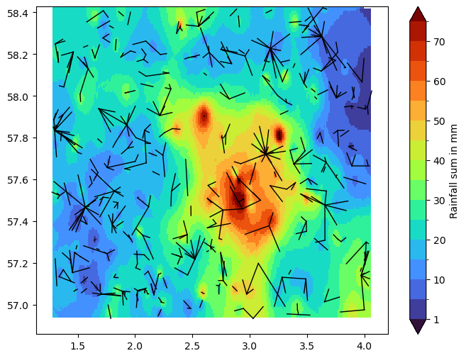
Next, we interpolate and plot a rainfall map of the rainfall sum over the full period of our dataset.
Note that we leave out CMLs with a wet_fraction > 0.3 because, as we have analyzed above, these contain a lot of erratic fluctuations. Also note that this is a primitive way of filtering out CMLs with erratic fluctuations. There are better ones, but we want to use something very simple here. If you want you can experiment here with different thresholds and investigate the effect on the resulting rainfall map.
[26]:
def plot_cml_lines(ds_cmls, ax):
    ax.plot(
        [ds_cmls.site_a_longitude, ds_cmls.site_b_longitude],
        [ds_cmls.site_a_latitude, ds_cmls.site_b_latitude],
        'k',
        linewidth=1,
    )

R_grid = idw_interpolator(
    x=cmls_R_1h.lon_center,
    y=cmls_R_1h.lat_center,
    z=cmls_R_1h.R.isel(channel_id=1).sum(dim='time').where(ds_cmls.wet_fraction < 0.3),
    resolution=0.01,
)

bounds = np.arange(0, 80, 5.0)
bounds[0] = 1
norm = mpl.colors.BoundaryNorm(boundaries=bounds, ncolors=256, extend='both')

fig, ax = plt.subplots(figsize=(8, 6))
pc = plt.pcolormesh(
    idw_interpolator.xgrid,
    idw_interpolator.ygrid,
    R_grid,
    shading='nearest',
    cmap='turbo',
    norm=norm,
)
plot_cml_lines(cmls_R_1h, ax=ax)
fig.colorbar(pc, label='Rainfall sum in mm');
Plot 1-hour rainfall maps for a selected period.
Note that this period was selected manually here and is selected based on the index-offset i + 88.
[27]:
fig, ax = plt.subplots(3, 3, sharex=True, sharey=True, figsize=(10, 10))

bounds = [0.1, 0.2, 0.5, 1, 2, 4, 7, 10, 20]
norm = mpl.colors.BoundaryNorm(boundaries=bounds, ncolors=256, extend='both')
cmap = plt.get_cmap('turbo').copy()
cmap.set_under('w')

for i, axi in enumerate(ax.flat):
    R_grid = idw_interpolator(
        x=cmls_R_1h.lon_center,
        y=cmls_R_1h.lat_center,
        z=cmls_R_1h.R.isel(channel_id=1).isel(time=i + 88).where(ds_cmls.wet_fraction < 0.3),
        resolution=0.01,
    )
    pc = axi.pcolormesh(
        idw_interpolator.xgrid,
        idw_interpolator.ygrid,
        R_grid,
        shading='nearest',
        cmap=cmap,
        norm=norm,
    )
    axi.set_title(str(cmls_R_1h.time.values[i + 88])[:19])

    plot_cml_lines(cmls_R_1h, ax=axi)

fig.subplots_adjust(right=0.9)
cbar_ax = fig.add_axes([0.95, 0.15, 0.02, 0.7])
cb = fig.colorbar(pc, cax=cbar_ax, label='Hourly rainfall sum in mm', );

[ ]: