Compare interpolation methods

In this notebook we do spatial interpolation of CML rainfall data and compare IDW and Kriging, each with different parameters. Before we can do the spatial interpolation we first have to process the example CML data.

[1]:

import pycomlink as pycml
import matplotlib.pyplot as plt
import matplotlib as mpl
import numpy as np
import pandas as pd
import xarray as xr

/Users/chwala-c/code/pycomlink/pycomlink/io/examples.py:1: UserWarning: pkg_resources is deprecated as an API. See https://setuptools.pypa.io/en/latest/pkg_resources.html. The pkg_resources package is slated for removal as early as 2025-11-30. Refrain from using this package or pin to Setuptools<81.
  import pkg_resources

Set fill values to NaN and interpolate short gaps

[ ]:

cmls['tsl'] = cmls.tsl.where(cmls.tsl != 255.0)
cmls['rsl'] = cmls.rsl.where(cmls.rsl != -99.9)
cmls['trsl'] = cmls.tsl - cmls.rsl

cmls['trsl'] = cmls.trsl.interpolate_na(dim='time', method='linear', max_gap='5min')

Do standard processing

We do a standard processing in this notebook without any explanation to quickly get CML rainfall estimates for interpolaton. For more details on the processing, check out the notebook on the basic CML processing workflow.

[4]:

cmls['wet'] = cmls.trsl.rolling(time=60, center=True).std(skipna=False) > 0.8

cmls['wet_fraction'] = (cmls.wet==1).sum(dim='time') / len(cmls.time)

cmls['baseline'] = pycml.processing.baseline.baseline_constant(
    trsl=cmls.trsl,
    wet=cmls.wet,
    n_average_last_dry=5,
)
cmls['waa'] = pycml.processing.wet_antenna.waa_schleiss_2013(
    rsl=cmls.trsl,
    baseline=cmls.baseline,
    wet=cmls.wet,
    waa_max=2.2,
    delta_t=1,
    tau=15,
)
cmls['A'] = cmls.trsl - cmls.baseline - cmls.waa

cmls['A'].values[cmls.A < 0] = 0

cmls['R'] = pycml.processing.k_R_relation.calc_R_from_A(
    A=cmls.A, L_km=cmls.length.values.astype('float'), f_GHz=cmls.frequency/1e9, pol=cmls.polarization
)

Calculate center point of each CML

We need this for the simple interpolatoin approaches that are used in this notebook which do simple interpolation of the rainfall values based on the center point of each CML.

[6]:

cmls_R_1h['lat_center'] = (cmls_R_1h.site_a_latitude + cmls_R_1h.site_b_latitude)/2
cmls_R_1h['lon_center'] = (cmls_R_1h.site_a_longitude + cmls_R_1h.site_b_longitude)/2

Function definition for quick plotting of CML paths

[7]:

def plot_cml_lines(ds_cmls, ax):
    ax.plot(
        [ds_cmls.site_a_longitude, ds_cmls.site_b_longitude],
        [ds_cmls.site_a_latitude, ds_cmls.site_b_latitude],
        'k',
        linewidth=1,
    )

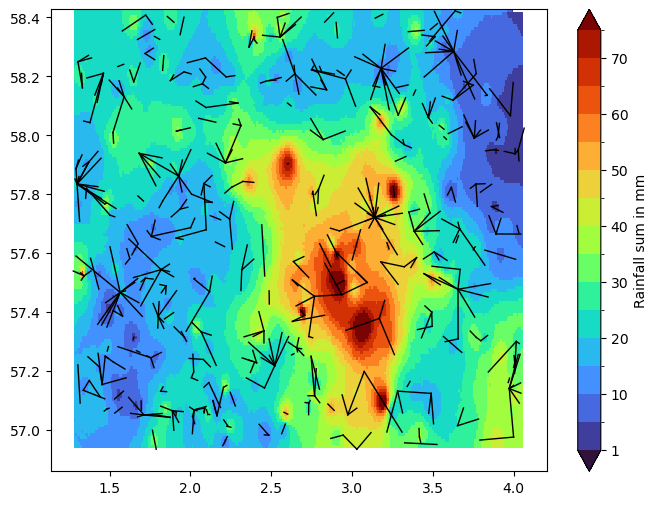
Do interpolation with IDW for rainfall sum per CML over example period

The folowing cell prepares the interpolator object.

[8]:

idw_interpolator = pycml.spatial.interpolator.IdwKdtreeInterpolator(
    nnear=15,
    p=2,
    exclude_nan=True,
    max_distance=0.3,
)

Do the interpolation by calling the interpolator object.

[9]:

R_grid = idw_interpolator(
    x=cmls_R_1h.lon_center,
    y=cmls_R_1h.lat_center,
    z=cmls_R_1h.R.isel(channel_id=1).sum(dim='time').where(cmls.isel(channel_id=1).wet_fraction < 0.3),
    resolution=0.01,
)

[10]:

bounds = np.arange(0, 80, 5.0)
bounds[0] = 1
norm = mpl.colors.BoundaryNorm(boundaries=bounds, ncolors=256, extend='both')

fig, ax = plt.subplots(figsize=(8, 6))
pc = plt.pcolormesh(
    idw_interpolator.xgrid,
    idw_interpolator.ygrid,
    R_grid,
    shading='nearest',
    cmap='turbo',
    norm=norm,
)
plot_cml_lines(cmls_R_1h, ax=ax)
fig.colorbar(pc, label='Rainfall sum in mm');

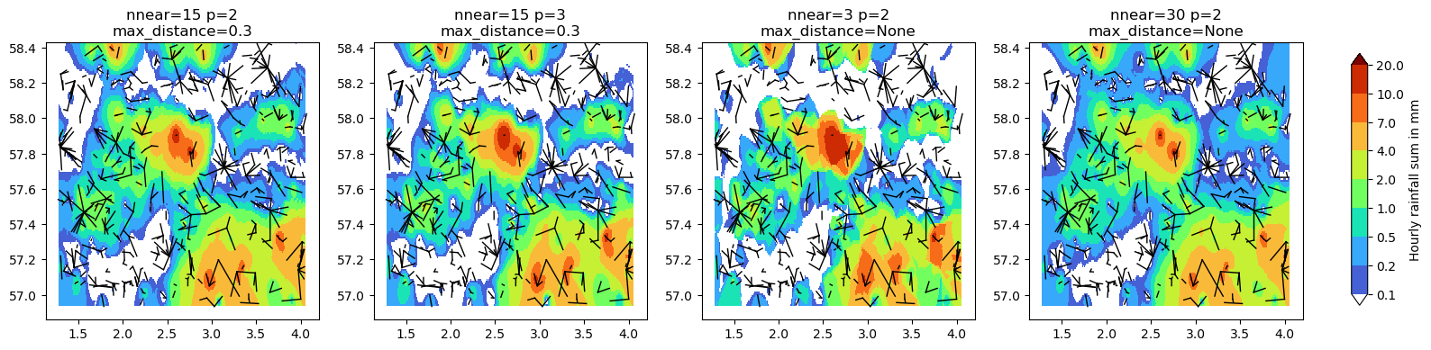
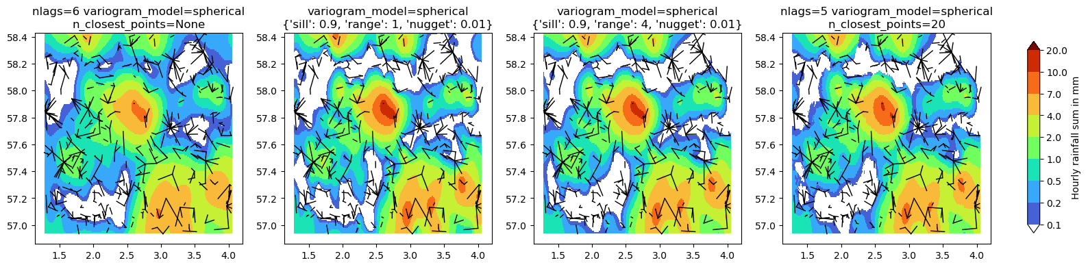
../_images/notebooks_Compare_interpolation_methods_20_0.png

Compare IDW and Kriging for different parameters

Here we use CML rainfall sum for one hour. Note that we exclude (by setting their result to NaN) CMLs that have a too high (0.3) wet_fraction.

[11]:

cmls_hour_selected = cmls_R_1h.R.isel(channel_id=1).isel(time=92).where(cmls.isel(channel_id=1).wet_fraction < 0.3)

The following cell defines the plotting functions and the colorscale

[12]:

bounds = [0.1, 0.2, 0.5, 1, 2, 4, 7, 10, 20]
norm = mpl.colors.BoundaryNorm(boundaries=bounds, ncolors=256, extend='both')
cmap = plt.get_cmap('turbo').copy()
cmap.set_under('w')


def idw_interpolate_and_plot(ax, nnear=15, p=2, max_distance=0.3):

    idw_interpolator = pycml.spatial.interpolator.IdwKdtreeInterpolator(
        nnear=nnear,
        p=p,
        exclude_nan=True,
        max_distance=max_distance,
    )

    R_grid = idw_interpolator(
        x=cmls_R_1h.lon_center,
        y=cmls_R_1h.lat_center,
        z=cmls_hour_selected,
        resolution=0.01,
    )

    pc = ax.pcolormesh(
        idw_interpolator.xgrid,
        idw_interpolator.ygrid,
        R_grid,
        shading='nearest',
        cmap=cmap,
        norm=norm,
    )
    ax.set_title(f'nnear={nnear} p={p}\nmax_distance={max_distance}')

    plot_cml_lines(cmls_R_1h, ax=ax)
    return pc


def kriging_interpolate_and_plot(
    ax,
    nlags=6,
    variogram_model='spherical',
    n_closest_points=None,
    variogram_parameters=None,
):

    kriging_interpolator = pycml.spatial.interpolator.OrdinaryKrigingInterpolator(
        nlags=nlags,
        variogram_model=variogram_model,
        variogram_parameters=variogram_parameters,
        weight=True,
        n_closest_points=n_closest_points,
    )

    R_grid = kriging_interpolator(
        x=cmls_R_1h.lon_center,
        y=cmls_R_1h.lat_center,
        z=cmls_hour_selected,
        resolution=0.01,
    )

    pc = ax.pcolormesh(
        idw_interpolator.xgrid,
        idw_interpolator.ygrid,
        R_grid,
        shading='nearest',
        cmap=cmap,
        norm=norm,
    )
    if variogram_parameters is None:
        ax.set_title(f'nlags={nlags} variogram_model={variogram_model}\nn_closest_points={n_closest_points}')
    else:
        ax.set_title(f'variogram_model={variogram_model}\n{variogram_parameters}')

    plot_cml_lines(cmls_R_1h, ax=ax)
    return pc

The code below plots 4 different variants of IDW and Kriging using different parameters.

[13]:

fig, axs = plt.subplots(1, 4, figsize=(18, 4))

idw_interpolate_and_plot(ax=axs[0], nnear=15, p=2, max_distance=0.3)
idw_interpolate_and_plot(ax=axs[1], nnear=15, p=3, max_distance=0.3)
idw_interpolate_and_plot(ax=axs[2], nnear=3, p=2, max_distance=None)
pc = idw_interpolate_and_plot(ax=axs[3], nnear=30, p=2, max_distance=None)

fig.subplots_adjust(right=0.9)
cbar_ax = fig.add_axes([0.93, 0.15, 0.01, 0.7])
cb = fig.colorbar(pc, cax=cbar_ax, label='Hourly rainfall sum in mm', );


fig, axs = plt.subplots(1, 4, figsize=(18, 4))

kriging_interpolate_and_plot(ax=axs[0])
kriging_interpolate_and_plot(ax=axs[1], variogram_parameters={'sill': 0.9, 'range': 1, 'nugget': 0.01})
kriging_interpolate_and_plot(ax=axs[2], variogram_parameters={'sill': 0.9, 'range': 4, 'nugget': 0.01})
pc = kriging_interpolate_and_plot(ax=axs[3], nlags=5, variogram_model='spherical', n_closest_points=20)

fig.subplots_adjust(right=0.9)
cbar_ax = fig.add_axes([0.93, 0.15, 0.01, 0.7])
cb = fig.colorbar(pc, cax=cbar_ax, label='Hourly rainfall sum in mm', );

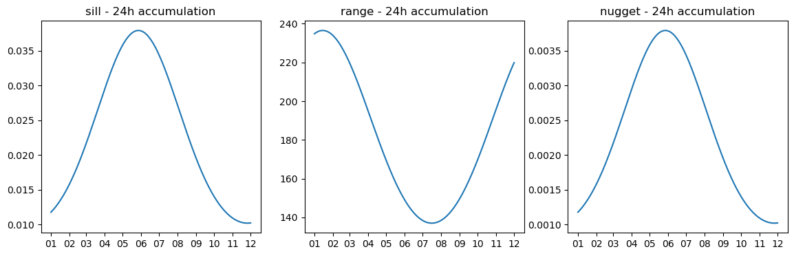
../_images/notebooks_Compare_interpolation_methods_26_0.png

../_images/notebooks_Compare_interpolation_methods_26_1.png

Generate Kriging parameters based on climatological variograms obtained in the Netherlands

This is based on the variograms obtained in Van de Beek et al., 2012 and the R implementation in RAINLINK by Overeem et al., 2016.

Plot sill, range and nugget for 24h rainfal accumulation

[14]:

# note that the year does not matter here, we only use the julian day inside the function
date_range = pd.date_range('2022-01-01', '2022-12-01', freq='D')

variogram_param_dict_list = []
for date in date_range:
    variogram_param_dict_list.append(pycml.spatial.interpolator.clim_var_param(date_str=date, time_scale_hours=24))

fig, axs = plt.subplots(1, 3, figsize=(14, 4))
for i, var_name in enumerate(['sill', 'range', 'nugget']):
    axs[i].plot(date_range, [variogram_param_dict[var_name] for variogram_param_dict in variogram_param_dict_list])
    axs[i].set_title(f"{var_name} - 24h accumulation")
    axs[i].xaxis.set_major_locator(mpl.dates.MonthLocator(bymonth=range(1,13,1)))
    axs[i].xaxis.set_major_formatter(mpl.dates.DateFormatter('%m'))

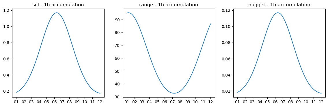
../_images/notebooks_Compare_interpolation_methods_29_0.png

Plot sill, range and nugget for 1h rainfall accumulation

[15]:

# note that the year does not matter here, we only use the julian day inside the function
date_range = pd.date_range('2022-01-01', '2022-12-01', freq='D')

variogram_param_dict_list = []
for date in date_range:
    variogram_param_dict_list.append(pycml.spatial.interpolator.clim_var_param(date_str=date, time_scale_hours=1))

fig, axs = plt.subplots(1, 3, figsize=(14, 4))
for i, var_name in enumerate(['sill', 'range', 'nugget']):
    axs[i].plot(date_range, [variogram_param_dict[var_name] for variogram_param_dict in variogram_param_dict_list])
    axs[i].set_title(f"{var_name} - 1h accumulation")
    axs[i].xaxis.set_major_locator(mpl.dates.MonthLocator(bymonth=range(1,13,1)))
    axs[i].xaxis.set_major_formatter(mpl.dates.DateFormatter('%m'))

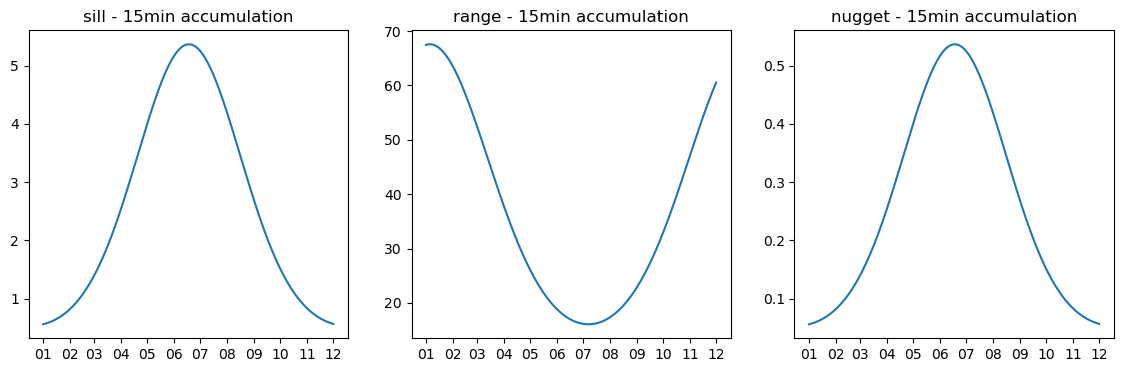
../_images/notebooks_Compare_interpolation_methods_31_0.png

We can also extrapolate for sub-hourly data, e.g. 15 minutes. Note that this is not covered in the original publication by van de Beek et al., 2012 but is also available in the original RAINLINK R code from Overeem et al., 2016.

[16]:

# note that the year does not matter here, we only use the julian day inside the function
date_range = pd.date_range('2022-01-01', '2022-12-01', freq='D')

variogram_param_dict_list = []
for date in date_range:
    variogram_param_dict_list.append(pycml.spatial.interpolator.clim_var_param(date_str=date, time_scale_hours=0.25))

fig, axs = plt.subplots(1, 3, figsize=(14, 4))
for i, var_name in enumerate(['sill', 'range', 'nugget']):
    axs[i].plot(date_range, [variogram_param_dict[var_name] for variogram_param_dict in variogram_param_dict_list])
    axs[i].set_title(f"{var_name} - 15min accumulation")
    axs[i].xaxis.set_major_locator(mpl.dates.MonthLocator(bymonth=range(1,13,1)))
    axs[i].xaxis.set_major_formatter(mpl.dates.DateFormatter('%m'))

../_images/notebooks_Compare_interpolation_methods_33_0.png

[ ]: